Data Handling
Class XI IP · Class XII IP

Data Handling

Store data in NumPy arrays and Pandas tables, pick out exactly the rows you want, and turn them into charts.

5 chapters18 topics11-IP · NumPy chapter12-IP · Unit 1
NUMPYfast arrays SERIES1-D, labelled DATAFRAME2-D table SELECTloc · iloc PLOTline·bar·hist SAVEcsv · png read_csv() loads a CSV file straight into a DataFrame, and to_csv() writes one back.
loc[1:3]
Includes row 3
iloc[1:3] stops before position 3
head()
5 rows by default
Same for tail(); pass a number for more or fewer
NaN
Unmatched labels
S1 + S2 gives NaN where a label is in only one
axis=1
Means columns
drop(…, axis=1) removes a column; axis=0, a row
Chapter 1 of 5 · NPY

NumPy

NumPy is the library that gives Python fast arrays of numbers. Pandas is built on top of it, so this is where data handling starts.

    NPY.01 · NumPy

    Introduction to NumPy

    11-IP

    NumPy (Numerical Python) is a library for working with arrays: grids of values that are all of the same type. Its array is called an ndarray (n-dimensional array). It is installed with pip install numpy and is almost always imported as np.

    • All elements have one data type, so NumPy stores them close together in memory and works on them very fast.
    • An operation on an array applies to every element at once. A list does not behave this way.
    Python
    import numpy as np
    L = [10, 20, 30]
    A = np.array(L)
    print(L * 2)
    print(A * 2)
    print(type(A))
    Output
    [10, 20, 30, 10, 20, 30] [20 40 60] <class 'numpy.ndarray'>
    ListNumPy array
    Element typesCan be mixedAll the same
    * 2 meansRepeat the listMultiply every element
    Speed and memorySlower, more memoryFaster, less memory
    NPY.02 · NumPy

    Creation of NumPy Arrays from List

    11-IP

    Pass a list to np.array(). A list of lists makes a 2-D array (rows and columns).

    Python
    import numpy as np
    a = np.array([4, 7, 1, 9])
    b = np.array([[1, 2, 3], [4, 5, 6]])
    print(a)
    print(b)
    print(b.shape, b.ndim, b.size, b.dtype)
    Output
    [4 7 1 9] [[1 2 3] [4 5 6]] (2, 3) 2 6 int64
    AttributeGivesFor b
    shape(rows, columns)(2, 3)
    ndimNumber of dimensions2
    sizeTotal number of elements6
    dtypeType of the elementsint64 (int32 on some Windows computers)

    If the list mixes types, NumPy converts everything to one type that can hold them all: integers with a float become floats, and anything with a string becomes strings.

    Python
    import numpy as np
    print(np.array([1, 2.5, 3]))
    print(np.array([1, 'two', 3]))
    Output
    [1. 2.5 3. ] ['1' 'two' '3']
    Common mistake

    NumPy prints arrays with spaces, not commas: [20 40 60], not [20, 40, 60]. Write it that way in "write the output" answers.

    Chapter practice · NPY

    Check your understanding

    What does np.array([1, 2, 3]) * 3 give?
    For a = np.array([[1, 2], [3, 4], [5, 6]]), a.shape is:
    np.array([2, 4.5]) stores its values as:
    Your score
    – / 3
    Answer every question to see your score.

    One-page revision

    import numpy as npthe usual import
    np.array(list)list → ndarray
    Same typemixed values are converted
    shape · ndim · size(rows, cols) · dimensions · count
    Chapter 2 of 5 · LIB

    Introduction to Python Libraries

    A library is a collection of ready-made code you import instead of writing it yourself. This unit uses two: Pandas for tables of data, and Matplotlib for charts.

      LIB.01 · Introduction to Python Libraries

      Pandas

      12-IP

      Pandas (from "panel data") is a library for storing, cleaning and analysing data in rows and columns, like a spreadsheet you control with code. Install it with pip install pandas and import it as pd.

      Data structures: Series and DataFrame #series-and-dataframes

      A Series is one column: values with a label (index) for each. A DataFrame is a table: several columns that share one row index. Each column of a DataFrame is a Series.

      SeriesDataFrame
      Dimensions1-D (one column)2-D (rows and columns)
      LabelsRow index onlyRow index and column names
      Data typesOne type for all valuesEach column can have its own type
      Mutability (CBSE terms)Value mutable, size immutableValue and size mutable
      NumPy ndarrayPandas DataFrame
      LabelsPositions only (0, 1, 2 …)Named rows and columns
      Data typesOne type for the whole arrayA different type per column
      Missing valuesNo special supportShown and handled as NaN
      LIB.02 · Introduction to Python Libraries

      Matplotlib

      12-IP

      Matplotlib is a library for drawing charts and graphs. Its pyplot module has one simple function for each part of a chart. Install it with pip install matplotlib and import pyplot as plt:

      Python
      import matplotlib.pyplot as plt

      Every chart follows three steps: prepare the data, plot it (plt.plot(), plt.bar(), plt.hist()), then show or save it (plt.show(), plt.savefig()). Chapter 5 covers each step.

      Chapter practice · LIB

      Check your understanding

      Which statement imports pyplot in the usual way?
      A Pandas structure with rows and columns, where each column may have a different type, is a:
      In CBSE terms, a Series is:
      Your score
      – / 3
      Answer every question to see your score.

      One-page revision

      import pandas as pdtables of data
      Series1-D, labelled; one type
      DataFrame2-D; a type per column
      import matplotlib.pyplot as pltcharts
      Chapter 3 of 5 · SER

      Series

      How to create a Series, do arithmetic with it, and pick out exactly the values you want. Every output below is what Python actually prints.

        SER.01 · Series

        Creation of Series

        12-IP

        Use pd.Series(data, index=…). If you give no index, Pandas numbers the values 0, 1, 2 …. The last line, dtype, tells you the type of the values.

        Python
        import pandas as pd
        marks = pd.Series([85, 90, 75])
        print(marks)
        Output
        0 85 1 90 2 75 dtype: int64
        Python · own index
        import pandas as pd
        marks = pd.Series([85, 90, 75],
                          index=['Asha', 'Kabir', 'Meera'])
        print(marks)
        Output
        Asha 85 Kabir 90 Meera 75 dtype: int64

        From an ndarray #from-ndarray

        Python
        import numpy as np
        import pandas as pd
        temps = np.array([31, 28, 29])
        s = pd.Series(temps, index=['Sun', 'Mon', 'Tue'])
        print(s)
        Output
        Sun 31 Mon 28 Tue 29 dtype: int64

        The index must have the same length as the array, otherwise you get a ValueError.

        From a dictionary #from-dictionary

        The keys become the index and the values become the data.

        Python
        import pandas as pd
        stock = {'Pens': 150, 'Erasers': 80,
                 'Notebooks': 200}
        inventory = pd.Series(stock)
        print(inventory)
        Output
        Pens 150 Erasers 80 Notebooks 200 dtype: int64

        From a scalar value #from-scalar

        A single value is repeated once for every label, so the index is required.

        Python
        import pandas as pd
        s = pd.Series(5, index=['a', 'b', 'c'])
        print(s)
        Output
        a 5 b 5 c 5 dtype: int64

        Series attributes

        An attribute is a property of the Series that you read without brackets: s.size, not s.size(). The examples use a Series of six students' marks (the same one used in SER.04).

        AttributeGivesFor the marks Series
        indexThe labelsIndex(['Asha', …, 'Tara'])
        valuesThe data as a NumPy array[45 78 62 91 55 83]
        dtypeType of the valuesint64
        shapeA tuple with the length(6,)
        sizeNumber of values, counting NaN6
        ndimNumber of dimensions: always 11
        nameA name for the Series (shown under it)None until you set it
        index.nameA name for the index (shown above it)None until you set it
        emptyTrue if the Series has no valuesFalse
        hasnansTrue if any value is NaNFalse
        Python
        import pandas as pd
        marks = [45, 78, 62, 91, 55, 83]
        names = ['Asha', 'Kabir', 'Meera',
                 'Ravi', 'Sana', 'Tara']
        s = pd.Series(marks, index=names)
        
        print(s.dtype)
        print(s.shape)
        print(s.size)
        print(s.ndim)
        print(s.empty)
        print(s.hasnans)
        Output
        int64 (6,) 6 1 False False

        name and index.name can be set; they then appear when the Series is printed:

        Python
        s.name = 'Marks'
        s.index.name = 'Student'
        print(s)
        Output
        Student Asha 45 Kabir 78 Meera 62 Ravi 91 Sana 55 Tara 83 Name: Marks, dtype: int64

        size counts every value; the method count() counts only values that are not NaN. A Series with NaN becomes float, as here.

        Python
        import pandas as pd
        r = pd.Series([4, None, 6])
        print(r)
        print(r.size, r.count(), r.hasnans)
        Output
        0 4.0 1 NaN 2 6.0 dtype: float64 3 2 True
        Python · an empty Series
        import pandas as pd
        e = pd.Series(dtype='int64')
        print(e.empty, e.size)
        Output
        True 0
        Exam tip

        shape of a Series is a tuple with one number and a comma, (6,). Writing 6 or (6) loses the mark.

        SER.02 · Series

        Mathematical Operations on Series

        12-IP

        + - * / between two Series work label by label, not position by position. Pandas lines up matching index labels. A label found in only one Series gets NaN (Not a Number), meaning "missing".

        Python
        import pandas as pd
        S1 = pd.Series([10, 20], index=['a', 'b'])
        S2 = pd.Series([30, 40], index=['b', 'c'])
        print(S1 + S2)
        Output
        a NaN b 50.0 c NaN dtype: float64

        Only b is in both, so only b gets a value. The result becomes float64, because NaN is a float. To treat missing values as 0, use the method form with fill_value. Arithmetic with a single number applies to every value.

        Python
        import pandas as pd
        S1 = pd.Series([10, 20], index=['a', 'b'])
        S2 = pd.Series([30, 40], index=['b', 'c'])
        print(S1.add(S2, fill_value=0))
        print(S1 * 2)
        Output
        a 10.0 b 50.0 c 40.0 dtype: float64 a 20 b 40 dtype: int64
        OperatorMethodWith missing values as 0
        S1 + S2S1.add(S2)S1.add(S2, fill_value=0)
        S1 - S2S1.sub(S2)S1.sub(S2, fill_value=0)
        S1 * S2S1.mul(S2)S1.mul(S2, fill_value=0)
        S1 / S2S1.div(S2)S1.div(S2, fill_value=0)
        Exam tip

        In "write the output" for S1 + S2, list every label from both Series in sorted order, write NaN for the unmatched ones, and end with dtype: float64.

        SER.03 · Series

        Head and Tail Functions

        12-IP

        head(n) #head

        Returns the first n values. With no number, n = 5.

        tail(n) #tail

        Returns the last n values. With no number, n = 5.

        Python
        import pandas as pd
        s = pd.Series([12, 45, 7, 30, 18, 60, 25])
        print(s.head())
        print(s.tail(2))
        Output
        0 12 1 45 2 7 3 30 4 18 dtype: int64 5 60 6 25 dtype: int64
        SER.04 · Series

        Selection, Indexing and Slicing

        12-IP

        This is the most-asked topic in the unit. Every example below uses the same Series of marks, so you can check each answer against it.

        The Series used below
        import pandas as pd
        marks = [45, 78, 62, 91, 55, 83]
        names = ['Asha', 'Kabir', 'Meera',
                 'Ravi', 'Sana', 'Tara']
        s = pd.Series(marks, index=names)
        print(s)
        Output
        Asha 45 Kabir 78 Meera 62 Ravi 91 Sana 55 Tara 83 dtype: int64
        POSITIONLABELVALUE0 · -6'Asha'451 · -5'Kabir'782 · -4'Meera'623 · -3'Ravi'914 · -2'Sana'555 · -1'Tara'83 s.iloc[2]by position s.loc['Meera']by label both give 62
        Every value has a label you choose and a position Pandas counts from 0 (or from -1 at the end). loc uses labels; iloc uses positions.

        1 · One value

        Give one label in square brackets, or use .loc[label], or use .iloc[position]. You get the value itself, not a Series.

        Python
        print(s['Meera'])
        print(s.loc['Meera'])
        print(s.iloc[2])
        Output
        62 62 62

        For labels that are valid Python names, s.Meera also works, but the bracket form always works.

        2 · Several values

        Put a list inside the brackets, so there are two pairs: s[['Ravi', 'Asha']]. The result is a Series in the order you listed, and a label or position may repeat.

        Python
        print(s[['Ravi', 'Asha']])
        print(s.iloc[[0, 3, 0]])
        Output
        Ravi 91 Asha 45 dtype: int64 Asha 45 Ravi 91 Asha 45 dtype: int64

        3 · Slicing by label: the end is included

        s['Kabir':'Ravi'] or s.loc['Kabir':'Ravi'] gives everything from Kabir up to and including Ravi. Leave out the start or the end to go from the beginning or to the end.

        Python
        print(s['Kabir':'Ravi'])
        print(s.loc[:'Kabir'])
        print(s.loc['Sana':])
        Output
        Kabir 78 Meera 62 Ravi 91 dtype: int64 Asha 45 Kabir 78 dtype: int64 Sana 55 Tara 83 dtype: int64

        4 · Slicing by position: the end is left out

        s.iloc[1:4] works like slicing a list: positions 1, 2 and 3, not 4. Negative positions count from the end, so s.iloc[-2:] gives the last two.

        Python
        print(s.iloc[1:4])
        print(s.iloc[:2])
        print(s.iloc[-2:])
        Output
        Kabir 78 Meera 62 Ravi 91 dtype: int64 Asha 45 Kabir 78 dtype: int64 Sana 55 Tara 83 dtype: int64

        5 · Steps and reversing

        A third number is the step: [::2] takes every second value and [::-1] reverses. A label slice in the wrong order ('Ravi':'Kabir') gives an empty Series, not an error.

        Python
        print(s.iloc[::2])
        print(s.iloc[::-1])
        print(s.loc['Ravi':'Kabir'])
        Output
        Asha 45 Meera 62 Sana 55 dtype: int64 Tara 83 Sana 55 Ravi 91 Meera 62 Kabir 78 Asha 45 dtype: int64 Series([], dtype: int64)

        6 · The default index trap

        When a Series has the default labels 0, 1, 2 …, its labels and positions look the same, but slicing still follows different rules:

        Python
        import pandas as pd
        n = pd.Series([10, 20, 30, 40, 50])
        print(n[1:3])
        print(n.loc[1:3])
        print(n[2])
        print(n.iloc[-1])
        Output
        1 20 2 30 dtype: int64 1 20 2 30 3 40 dtype: int64 30 50
        On n (labels 0–4)UsesGives
        n[1:3]positions (a slice in plain brackets)2 values: labels 1, 2
        n.loc[1:3]labels, end included3 values: labels 1, 2, 3
        n[2]the label 230
        n[-1]the label -1, which doesn't existKeyError. Use n.iloc[-1]

        7 · Selecting by condition (boolean indexing)

        A comparison such as s > 80 gives a Series of True/False for every value. Put it inside s[…] and only the True values are kept, with their labels.

        Python
        print(s > 80)
        print(s[s > 80])
        Output
        Asha False Kabir False Meera False Ravi True Sana False Tara True dtype: bool Ravi 91 Tara 83 dtype: int64

        Join conditions with & (and), | (or), and ~ (not). Each condition needs its own brackets, and the words and / or do not work here.

        Python
        print(s[(s >= 60) & (s < 85)])
        print(s[(s < 50) | (s > 90)])
        print(s[~(s > 60)])
        Output
        Kabir 78 Meera 62 Tara 83 dtype: int64 Asha 45 Ravi 91 dtype: int64 Asha 45 Sana 55 dtype: int64

        8 · Changing values through a selection

        Anything you can select, you can also assign to. A Series is value mutable.

        Python
        s['Asha'] = 50
        s[s < 60] = 60
        print(s)
        Output
        Asha 60 Kabir 78 Meera 62 Ravi 91 Sana 60 Tara 83 dtype: int64

        Two attributes come up in selection questions: s.index gives the labels, and s.values gives the data as a NumPy array.

        Python
        print(s.index)
        print(s.values)
        print(s.size)
        Output
        Index(['Asha', 'Kabir', 'Meera', 'Ravi', 'Sana', 'Tara'], dtype='object') [45 78 62 91 55 83] 6

        Summary

        You writeSelects byEnd of sliceYou get
        s['Meera'], s.loc['Meera']labeln/aone value
        s.iloc[2]positionn/aone value
        s[['Ravi', 'Asha']], s.iloc[[0, 3]]list of labels / positionsn/aSeries
        s['Kabir':'Ravi'], s.loc[…:…]labelincludedSeries
        s.iloc[1:4]positionleft outSeries
        s[s > 80]conditionn/aSeries
        MistakeWhat happens
        A label that doesn't exist: s['Zoya']KeyError
        A position past the end: s.iloc[10]IndexError
        s['Ravi', 'Asha'] (one pair of brackets)KeyError: use a list, s[['Ravi', 'Asha']]
        s[s > 50 and s < 80]ValueError: use (s > 50) & (s < 80)
        Exam tip

        Older papers write s[0] on a Series with name labels to mean "the first value". It still works in Pandas 2 but warns that it is being removed. Write s.iloc[0] in your answers.

        Chapter practice · SER

        Check your understanding

        Predict the output

        import pandas as pd
        print(pd.Series(5, index=[0, 1, 2]))
        import pandas as pd
        s = pd.Series([11, 22, 33, 44],
                      index=['a', 'b', 'c', 'd'])
        print(s[s % 2 != 0])
        import pandas as pd
        s = pd.Series([5, 10, 15, 20, 25])
        print(s[1:3])
        print(s.loc[1:3])
        import pandas as pd
        S1 = pd.Series([10, 20], index=['a', 'b'])
        S2 = pd.Series([30, 40], index=['b', 'c'])
        print(S1 + S2)
        import pandas as pd
        s = pd.Series([3, 6, 9, 12],
                      index=['w', 'x', 'y', 'z'])
        print(s['x':'z'])
        print(s.iloc[1:3])
        import pandas as pd
        s = pd.Series([10, 20, 30], index=[3, 2, 1])
        print(s.loc[2])
        print(s.iloc[2])
        import pandas as pd
        s = pd.Series([4, 8, 15, 16, 23])
        print(s.iloc[::-2])
        import pandas as pd
        s = pd.Series({'a': 1, 'b': 2, 'c': 3})
        s[s > 1] = 0
        print(s)

        Self-check quiz

        If two Series are added and some labels don't match, those labels get:
        With no number given, s.head() returns:
        To create a Series from a dictionary, the dictionary's keys become the:
        For s = pd.Series([5, 6, 7], index=['p', 'q', 'r']), s['p':'q'] gives:
        Which gives the last value of any Series s?
        To keep values between 50 and 80 (inclusive):
        For s = pd.Series([10, 20, 30, 40]), s.shape is:
        A Series has 5 values, one of them NaN. s.size and s.count() are:
        s.values returns:
        Your score
        – / 9
        Answer every question to see your score.

        One-page revision

        pd.Series(list)index 0, 1, 2 …
        index=[…]your own labels; same length
        Series(dict)keys → index
        Series(5, index=…)scalar repeated; index needed
        S1 + S2by label; unmatched → NaN
        fill_value=0treat missing as 0
        head() / tail()first / last 5
        s['a':'c']label slice, end included
        s.iloc[0:2]position slice, end left out
        s[s > 50]boolean indexing
        s[['a', 'c']]several labels: double brackets
        & · | · ~and · or · not, each in brackets
        s.iloc[-1]last value, always
        size vs count()all values / non-NaN only
        s.shape(n,): a one-item tuple
        name · index.namelabels shown when printed
        empty · hasnansno values? any NaN?
        s.loc['b':'a']wrong order → empty Series
        Chapter 4 of 5 · DF

        Data Frames

        Most board questions in this unit come from this chapter. Many examples use the file marks.csv, shown first, so you can follow each change.

          DF.01 · Data Frames

          Creation of Data Frames

          12-IP

          Use pd.DataFrame(data, index=…, columns=…). With no index, rows are numbered from 0.

          From a dictionary of Series #from-dict-of-series

          Each key becomes a column name, and each Series becomes that column.

          Python
          import pandas as pd
          city = pd.Series(['Delhi', 'Mumbai', 'Kolkata'])
          temp = pd.Series([32, 30, 28])
          df = pd.DataFrame({'City': city,
                             'Temperature': temp})
          print(df)
          Output
          City Temperature 0 Delhi 32 1 Mumbai 30 2 Kolkata 28

          From a list of dictionaries #from-list-of-dicts

          Each dictionary becomes one row; its keys become column names. A key missing from a dictionary gives NaN in that row.

          Python
          import pandas as pd
          d1 = {'acc': 98, 'bst': 95, 'eco': 88}
          d2 = {'acc': 94, 'bst': 87}
          d3 = {'acc': 89, 'bst': 76, 'eco': 81}
          df = pd.DataFrame([d1, d2, d3],
                            index=['Meet', 'Ram', 'Smita'])
          print(df)
          Output
          acc bst eco Meet 98 95 88.0 Ram 94 87 NaN Smita 89 76 81.0

          Ram has no eco, so it is NaN, and the whole eco column becomes float (88.0, 81.0).

          From a text / CSV file #from-csv

          A CSV (comma-separated values) file is plain text: one row per line, values separated by commas, with column names on the first line. pd.read_csv() turns it into a DataFrame.

          marks.csv
          RollNo,Name,Maths,Science 101,Asha,88,92 102,Kabir,74,81 103,Meera,91,85 104,Ravi,66,70
          Python → output
          import pandas as pd
          df = pd.read_csv('marks.csv')
          print(df)
          RollNo Name Maths Science 0 101 Asha 88 92 1 102 Kabir 74 81 2 103 Meera 91 85 3 104 Ravi 66 70
          DF.02 · Data Frames

          Display and Iteration

          12-IP

          Display #display

          print(df) shows the whole table. These attributes describe it (no brackets after them):

          Python
          import pandas as pd
          df = pd.read_csv('marks.csv')
          print(df.shape)
          print(df.size)
          print(df.columns)
          print(df.index)
          Output
          (4, 4) 16 Index(['RollNo', 'Name', 'Maths', 'Science'], dtype='object') RangeIndex(start=0, stop=4, step=1)
          Python
          import pandas as pd
          df = pd.read_csv('marks.csv')
          print(df.dtypes)
          print(df.ndim)
          print(df.empty)
          print(len(df))
          Output
          RollNo int64 Name object Maths int64 Science int64 dtype: object 2 False 4
          Python
          import pandas as pd
          df = pd.read_csv('marks.csv')
          print(df.values)
          Output
          [[101 'Asha' 88 92] [102 'Kabir' 74 81] [103 'Meera' 91 85] [104 'Ravi' 66 70]]

          T (transpose) swaps rows and columns, so the row labels become column names:

          Python
          import pandas as pd
          df = pd.read_csv('marks.csv')
          print(df.T)
          Output
          0 1 2 3 RollNo 101 102 103 104 Name Asha Kabir Meera Ravi Maths 88 74 91 66 Science 92 81 85 70

          axes gives both labels at once: the row index, then the columns. The method count() gives the number of non-NaN values in each column.

          Python
          import pandas as pd
          df = pd.DataFrame({'A': [1, None, 3], 'B': [4, 5, 6]})
          print(df.axes)
          print(df.count())
          Output
          [RangeIndex(start=0, stop=3, step=1), Index(['A', 'B'], dtype='object')] A 2 B 3 dtype: int64
          AttributeGivesFor marks.csv
          indexThe row labelsRangeIndex(start=0, stop=4, step=1)
          columnsThe column namesIndex(['RollNo', 'Name', 'Maths', 'Science'])
          axes[row index, columns] as a listboth of the above
          dtypesThe type of each columnint64, object, int64, int64
          valuesAll the data as a 2-D NumPy array4 rows × 4 values
          shape(rows, columns)(4, 4)
          sizerows × columns16
          ndimNumber of dimensions: always 22
          TThe transpose4 rows of RollNo, Name, Maths, Science
          emptyTrue if there are no valuesFalse
          len(df), df.count()Functions: number of rows; non-NaN values per column4; 4 each
          Exam tip

          shape vs size: shape is a tuple, (4, 4); size is one number, rows × columns = 16. Text columns have dtype object.

          Iteration #iteration

          iterrows() goes through the table row by row, giving each row's label and the row as a Series. items() goes column by column.

          Python · rows
          import pandas as pd
          df = pd.DataFrame({'Name': ['Asha', 'Kabir'],
                             'Maths': [88, 74]})
          for label, row in df.iterrows():
              print(label, row['Name'], row['Maths'])
          Output
          0 Asha 88 1 Kabir 74
          Python · columns
          import pandas as pd
          df = pd.DataFrame({'Name': ['Asha', 'Kabir'],
                             'Maths': [88, 74]})
          for col, values in df.items():
              print(col, list(values))
          Output
          Name ['Asha', 'Kabir'] Maths [88, 74]
          Note

          Older books use iteritems() for columns. It was removed in Pandas 2.0, so on a new computer use items(), which does the same job.

          DF.03 · Data Frames

          Operations on Rows and Columns

          12-IP

          Add #add

          To add a column, assign to a column name that doesn't exist yet: df['New'] = …. What you put on the right decides what goes in each row. All these start from marks.csv.

          1 · A list of values

          One value per row, in row order. The list must have exactly as many values as there are rows.

          Python
          import pandas as pd
          df = pd.read_csv('marks.csv')
          df['House'] = ['Red', 'Blue', 'Red', 'Green']
          print(df)
          Output
          RollNo Name Maths Science House 0 101 Asha 88 92 Red 1 102 Kabir 74 81 Blue 2 103 Meera 91 85 Red 3 104 Ravi 66 70 Green

          With 3 values for 4 rows you get ValueError: Length of values (3) does not match length of index (4).

          2 · A constant value

          A single value is copied into every row.

          Python
          import pandas as pd
          df = pd.read_csv('marks.csv')
          df['Class'] = 12
          df['School'] = 'KV'
          print(df)
          Output
          RollNo Name Maths Science Class School 0 101 Asha 88 92 12 KV 1 102 Kabir 74 81 12 KV 2 103 Meera 91 85 12 KV 3 104 Ravi 66 70 12 KV

          3 · From columns that already exist

          Arithmetic on whole columns works row by row, so a new column can be worked out from others. A comparison makes a column of True/False.

          Python
          import pandas as pd
          df = pd.read_csv('marks.csv')
          df['Total'] = df['Maths'] + df['Science']
          df['Percent'] = df['Total'] / 2
          df['Pass'] = df['Maths'] >= 70
          print(df)
          Output
          RollNo Name Maths Science Total Percent Pass 0 101 Asha 88 92 180 90.0 True 1 102 Kabir 74 81 155 77.5 True 2 103 Meera 91 85 176 88.0 True 3 104 Ravi 66 70 136 68.0 False

          4 · From a Series

          A Series is matched to the rows by index label, not by position. A row whose label isn't in the Series gets NaN (and the column becomes float); labels in the Series that aren't rows are ignored.

          Python
          import pandas as pd
          df = pd.read_csv('marks.csv')
          bonus = pd.Series([5, 3, 4], index=[0, 2, 3])
          df['Bonus'] = bonus
          print(df)
          Output
          RollNo Name Maths Science Bonus 0 101 Asha 88 92 5.0 1 102 Kabir 74 81 NaN 2 103 Meera 91 85 3.0 3 104 Ravi 66 70 4.0

          Row 1 (Kabir) has no bonus because label 1 isn't in bonus.

          5 · At a chosen position: insert()

          df['New'] = … always adds at the end. df.insert(position, name, values) puts the column where you want it and changes df directly. Using a name that already exists gives ValueError: cannot insert …, already exists.

          Python
          import pandas as pd
          df = pd.read_csv('marks.csv')
          df.insert(1, 'Section', ['A', 'B', 'A', 'B'])
          print(df)
          Output
          RollNo Section Name Maths Science 0 101 A Asha 88 92 1 102 B Kabir 74 81 2 103 A Meera 91 85 3 104 B Ravi 66 70

          6 · With loc

          df.loc[:, 'New'] = … means "all rows, column New" and does the same as df['New'] = ….

          Python
          import pandas as pd
          df = pd.read_csv('marks.csv')
          df.loc[:, 'Grade'] = ['A', 'B', 'A', 'C']
          print(df)
          Output
          RollNo Name Maths Science Grade 0 101 Asha 88 92 A 1 102 Kabir 74 81 B 2 103 Meera 91 85 A 3 104 Ravi 66 70 C

          Changing a column that already exists

          Assigning to an existing name replaces that column instead of adding a new one:

          Python
          import pandas as pd
          df = pd.read_csv('marks.csv')
          df['Maths'] = df['Maths'] + 5
          print(df)
          Output
          RollNo Name Maths Science 0 101 Asha 93 92 1 102 Kabir 79 81 2 103 Meera 96 85 3 104 Ravi 71 70
          WayExampleRule
          Listdf['House'] = ['Red', 'Blue', 'Red', 'Green']Length must equal the number of rows
          Constantdf['Class'] = 12Same value in every row
          Existing columnsdf['Total'] = df['Maths'] + df['Science']Worked out row by row
          Seriesdf['Bonus'] = bonusMatched by label; missing labels → NaN
          insert()df.insert(1, 'Section', […])At a position; name must be new
          locdf.loc[:, 'Grade'] = […]Same as df['Grade'] = …

          Adding a row

          Assign a list (one value per column, in column order) to a new label with loc:

          Python
          import pandas as pd
          df = pd.read_csv('marks.csv')
          df['Total'] = df['Maths'] + df['Science']
          df.loc[4] = [105, 'Sana', 79, 88, 167]
          print(df)
          Output
          RollNo Name Maths Science Total 0 101 Asha 88 92 180 1 102 Kabir 74 81 155 2 103 Meera 91 85 176 3 104 Ravi 66 70 136 4 105 Sana 79 88 167
          Note

          Older books add rows with df.append(), which was removed in Pandas 2.0. Use df.loc[label] = […] instead.

          Select #select

          One column in single brackets gives a Series; a list of columns in double brackets gives a DataFrame. Selecting rows, single values and rows by a condition is covered in full in DF.05 Indexing.

          Python
          import pandas as pd
          df = pd.read_csv('marks.csv')
          print(df['Name'])
          print(df[['Name', 'Maths']])
          Output
          0 Asha 1 Kabir 2 Meera 3 Ravi Name: Name, dtype: object Name Maths 0 Asha 88 1 Kabir 74 2 Meera 91 3 Ravi 66

          Delete #delete

          Pandas has three ways to delete: drop() for rows and columns (one or many), del for one column, and pop() for one column that you also want to keep. Most examples start from marks.csv.

          axis=1 · columns → axis=0 rows ↓ RollNoNameMathsScience0101Asha88921102Kabir74812103Meera91853104Ravi6670 df.drop(2) removes a row df.drop('Science', axis=1) removes a column
          axis=0 (the default) means rows, named by the index. axis=1 means columns. Forgetting axis=1 makes Pandas look for a row with that name.

          1 · drop() a column

          Give the column name and axis=1. drop() returns a new DataFrame and leaves the original unchanged: the last line shows that df still has Science.

          Python
          import pandas as pd
          df = pd.read_csv('marks.csv')
          
          new = df.drop('Science', axis=1)
          print(new)
          print(df.columns)
          Output
          RollNo Name Maths 0 101 Asha 88 1 102 Kabir 74 2 103 Meera 91 3 104 Ravi 66 Index(['RollNo', 'Name', 'Maths', 'Science'], dtype='object')

          2 · drop() several columns

          Pass a list of names. Writing columns=… is the same as giving names with axis=1, and is easier to read.

          Python
          import pandas as pd
          df = pd.read_csv('marks.csv')
          
          print(df.drop(['Maths', 'Science'], axis=1))
          print(df.drop(columns=['RollNo', 'Science']))
          Output
          RollNo Name 0 101 Asha 1 102 Kabir 2 103 Meera 3 104 Ravi Name Maths 0 Asha 88 1 Kabir 74 2 Meera 91 3 Ravi 66

          3 · drop() a row

          Give the row label. Rows are the default (axis=0), so no axis is needed. index=… says the same thing in words.

          Python
          import pandas as pd
          df = pd.read_csv('marks.csv')
          
          print(df.drop(2))
          print(df.drop(index=0))
          Output
          RollNo Name Maths Science 0 101 Asha 88 92 1 102 Kabir 74 81 3 104 Ravi 66 70 RollNo Name Maths Science 1 102 Kabir 74 81 2 103 Meera 91 85 3 104 Ravi 66 70

          4 · drop() several rows

          Pass a list of labels. The labels that are left stay as they were: here 0 and 2, not 0 and 1.

          Python
          import pandas as pd
          df = pd.read_csv('marks.csv')
          
          print(df.drop([1, 3]))
          Output
          RollNo Name Maths Science 0 101 Asha 88 92 2 103 Meera 91 85

          When the row labels are names, use the names. This uses the table from DF.05 (Asha, Kabir, Meera, Ravi):

          Python
          print(df.drop(['Kabir', 'Ravi']))
          Output
          Maths Science City Asha 88 92 Delhi Meera 91 85 Pune

          5 · drop() rows by position

          drop() takes labels, not positions. To delete the 1st and 3rd rows whatever their labels, look the labels up with df.index[[0, 2]]:

          Python
          print(df.index[[0, 2]])
          print(df.drop(df.index[[0, 2]]))
          Output
          Index(['Asha', 'Meera'], dtype='object') Maths Science City Kabir 74 81 Delhi Ravi 66 70 Agra

          6 · drop() rows that meet a condition

          Find the labels of the matching rows with a boolean selection and .index, then drop them. Keeping the other rows, df = df[df['Maths'] >= 75], gives the same result.

          Python
          import pandas as pd
          df = pd.read_csv('marks.csv')
          
          low = df[df['Maths'] < 75].index
          print(low)
          df = df.drop(low)
          print(df)
          Output
          Index([1, 3], dtype='int64') RollNo Name Maths Science 0 101 Asha 88 92 2 103 Meera 91 85

          7 · Rows and columns in one call

          Python
          import pandas as pd
          df = pd.read_csv('marks.csv')
          
          print(df.drop(index=[0, 3], columns=['RollNo']))
          Output
          Name Maths Science 1 Kabir 74 81 2 Meera 91 85

          8 · Making the change stick: inplace=True or assign back

          Either write df = df.drop(…), or write df.drop(…, inplace=True), which changes df itself and returns None. Never combine them: df = df.drop(…, inplace=True) sets df to None.

          Python
          import pandas as pd
          df = pd.read_csv('marks.csv')
          
          df.drop('RollNo', axis=1, inplace=True)
          print(df)
          result = df.drop(0, inplace=True)
          print(result)
          Output
          Name Maths Science 0 Asha 88 92 1 Kabir 74 81 2 Meera 91 85 3 Ravi 66 70 None

          9 · Renumbering after deleting rows

          Deleting rows leaves gaps in the labels. reset_index(drop=True) numbers the rows 0, 1, 2 … again. drop=True stops the old labels from being kept as a new column.

          Python
          import pandas as pd
          df = pd.read_csv('marks.csv')
          
          df = df.drop([0, 2])
          print(df)
          df = df.reset_index(drop=True)
          print(df)
          Output
          RollNo Name Maths Science 1 102 Kabir 74 81 3 104 Ravi 66 70 RollNo Name Maths Science 0 102 Kabir 74 81 1 104 Ravi 66 70

          10 · del: one column, permanently

          del df['Science'] removes the column from df at once. There is no inplace, nothing is returned, and it works on one column only. It cannot delete rows.

          Python
          import pandas as pd
          df = pd.read_csv('marks.csv')
          
          del df['Science']
          print(df)
          Output
          RollNo Name Maths 0 101 Asha 88 1 102 Kabir 74 2 103 Meera 91 3 104 Ravi 66

          11 · pop(): remove a column and keep it

          df.pop('Maths') removes the column from df and returns it as a Series, so you can still use it. Like del, it takes one column only.

          Python
          import pandas as pd
          df = pd.read_csv('marks.csv')
          
          m = df.pop('Maths')
          print(m)
          print(df)
          Output
          0 88 1 74 2 91 3 66 Name: Maths, dtype: int64 RollNo Name Science 0 101 Asha 92 1 102 Kabir 81 2 103 Meera 85 3 104 Ravi 70

          12 · Names that don't exist

          Dropping a label that isn't there raises KeyError: "['Hindi'] not found in axis". Add errors='ignore' to skip missing names and drop the rest:

          Python
          import pandas as pd
          df = pd.read_csv('marks.csv')
          
          print(df.drop(['Science', 'Hindi'], axis=1,
                        errors='ignore'))
          Output
          RollNo Name Maths 0 101 Asha 88 1 102 Kabir 74 2 103 Meera 91 3 104 Ravi 66

          drop vs del vs pop

          drop()del df['c']df.pop('c')
          DeletesRows or columnsOne columnOne column
          Several at once?Yes, with a listNoNo
          Changes df itself?Only with inplace=TrueYesYes
          ReturnsA new DataFrame (None with inplace)NothingThe removed column (Series)
          Missing nameKeyError, unless errors='ignore'KeyErrorKeyError
          MistakeWhat happens
          df.drop('Maths') (no axis=1)KeyError: it looks for a row labelled Maths
          df.drop('Maths', axis=1) and then using dfMaths is still there: assign back or use inplace=True
          df = df.drop(…, inplace=True)df becomes None
          del df[['Maths', 'Science']]Error: del takes one column. Use drop(columns=[…])
          del df.loc[0]Error: del cannot delete rows. Use df.drop(0)

          Rename #rename

          Give rename() a dictionary of old name: new name, for columns=, index=, or both.

          Python
          import pandas as pd
          df = pd.DataFrame({'A': ['P01', 'P02'],
                             'B': ['Pen', 'Pencil']})
          df = df.rename(columns={'A': 'PID', 'B': 'PNAME'})
          df = df.rename(index={0: 'x', 1: 'y'})
          print(df)
          Output
          PID PNAME x P01 Pen y P02 Pencil
          Exam tip

          "df.drop('Column1', axis=1) deletes the column permanently": false. Without inplace=True, df is unchanged.

          DF.04 · Data Frames

          Head and Tail Functions

          12-IP

          head(n) #head

          The first n rows; 5 if you give no number.

          tail(n) #tail

          The last n rows; 5 if you give no number. If the table has fewer rows than n, you simply get all of them.

          Python
          import pandas as pd
          df = pd.read_csv('marks.csv')
          print(df.head(2))
          print(df.tail(1))
          Output
          RollNo Name Maths Science 0 101 Asha 88 92 1 102 Kabir 74 81 RollNo Name Maths Science 3 104 Ravi 66 70
          DF.05 · Data Frames

          Indexing

          12-IP

          Selecting rows, columns and single values is asked in almost every paper. All the examples below use this table, which has name labels, so you can see clearly when a label is used and when a position is.

          The DataFrame used below
          import pandas as pd
          data = {'Maths':   [88, 74, 91, 66],
                  'Science': [92, 81, 85, 70],
                  'City':    ['Delhi', 'Delhi', 'Pune', 'Agra']}
          names = ['Asha', 'Kabir', 'Meera', 'Ravi']
          df = pd.DataFrame(data, index=names)
          print(df)
          Output
          Maths Science City Asha 88 92 Delhi Kabir 74 81 Delhi Meera 91 85 Pune Ravi 66 70 Agra

          Label indexing: columns, loc and iloc #loc-iloc

          012column positionposlabelMathsScienceCity0'Asha'8892Delhi1'Kabir'7481Delhi2'Meera'9185Pune3'Ravi'6670Agra df.loc['Kabir':'Meera', 'Maths':'Science'] is the same block as df.iloc[1:3, 0:2]
          Rows and columns both have a label and a position. Inside loc[…] and iloc[…], the part before the comma picks rows and the part after it picks columns.

          1 · Columns: df['…']

          Plain square brackets with a column name give that column as a Series. A list of names gives a DataFrame with those columns, in your order. df.Maths also works for simple names.

          Python
          print(df['Maths'])
          print(df[['City', 'Maths']])
          Output
          Asha 88 Kabir 74 Meera 91 Ravi 66 Name: Maths, dtype: int64 City Maths Asha Delhi 88 Kabir Delhi 74 Meera Pune 91 Ravi Agra 66

          2 · Rows by label: df.loc[…]

          One label gives that row as a Series, whose index is the column names and whose Name is the row label. A list of labels gives a DataFrame.

          Python
          print(df.loc['Kabir'])
          print(df.loc[['Asha', 'Ravi']])
          Output
          Maths 74 Science 81 City Delhi Name: Kabir, dtype: object Maths Science City Asha 88 92 Delhi Ravi 66 70 Agra

          3 · Rows by position: df.iloc[…]

          The same, but with positions 0, 1, 2 …; df.iloc[-1] is the last row.

          Python
          print(df.iloc[0])
          print(df.iloc[[0, 2]])
          Output
          Maths 88 Science 92 City Delhi Name: Asha, dtype: object Maths Science City Asha 88 92 Delhi Meera 91 85 Pune

          4 · A range of rows: three ways

          These three give the same rows here, but read the slice ends: loc includes 'Meera', while iloc[1:3] and df[1:3] stop before position 3. A slice in plain brackets picks rows, even though a name in plain brackets picks a column.

          Python
          print(df.loc['Kabir':'Meera'])
          print(df.iloc[1:3])
          print(df[1:3])
          Output
          Maths Science City Kabir 74 81 Delhi Meera 91 85 Pune Maths Science City Kabir 74 81 Delhi Meera 91 85 Pune Maths Science City Kabir 74 81 Delhi Meera 91 85 Pune

          5 · Rows and columns together

          Write rows, then a comma, then columns. One row and one column gives a single value. Slices and lists give a smaller DataFrame.

          Python
          print(df.loc['Meera', 'Maths'])
          print(df.loc['Kabir':'Ravi', 'Maths':'Science'])
          print(df.iloc[0:2, [0, 2]])
          Output
          91 Maths Science Kabir 74 81 Meera 91 85 Ravi 66 70 Maths City Asha 88 Delhi Kabir 74 Delhi

          Use : on its own to mean "all rows" (or all columns):

          Python
          print(df.loc[:, 'Science':'City'])
          print(df.iloc[:, 0])
          Output
          Science City Asha 92 Delhi Kabir 81 Delhi Meera 85 Pune Ravi 70 Agra Asha 88 Kabir 74 Meera 91 Ravi 66 Name: Maths, dtype: int64

          Boolean indexing #boolean-indexing

          A condition on a column, such as df['Maths'] > 80, gives True/False for every row. Put it inside df[…] to keep only the rows where it is True. This works for text columns too.

          Python
          print(df['Maths'] > 80)
          print(df[df['Maths'] > 80])
          print(df[df['City'] == 'Delhi'])
          Output
          Asha True Kabir False Meera True Ravi False Name: Maths, dtype: bool Maths Science City Asha 88 92 Delhi Meera 91 85 Pune Maths Science City Asha 88 92 Delhi Kabir 74 81 Delhi

          Join conditions with &, | and ~, each in its own brackets. Use loc to filter rows and pick columns at the same time. isin() checks for several values at once.

          Python
          print(df[(df['Maths'] > 70) & (df['Science'] > 82)])
          print(df.loc[df['Science'] < 85, ['Maths', 'City']])
          print(df[df['City'].isin(['Pune', 'Agra'])])
          Output
          Maths Science City Asha 88 92 Delhi Meera 91 85 Pune Maths City Kabir 74 Delhi Ravi 66 Agra Maths Science City Meera 91 85 Pune Ravi 66 70 Agra

          Changing values through a selection

          Assign to a loc selection to change one value, or every value that meets a condition.

          Python
          df.loc['Ravi', 'Maths'] = 70
          df.loc[df['Science'] < 85, 'Science'] = 85
          print(df)
          Output
          Maths Science City Asha 88 92 Delhi Kabir 74 85 Delhi Meera 91 85 Pune Ravi 70 85 Agra

          Summary

          You writePicksYou get
          df['Maths']one columnSeries
          df[['City', 'Maths']]several columnsDataFrame
          df.loc['Kabir'] / df.iloc[1]one rowSeries
          df.loc['Kabir':'Meera']rows by label, end includedDataFrame
          df.iloc[1:3], df[1:3]rows by position, end left outDataFrame
          df.loc['Meera', 'Maths'] / df.iloc[2, 0]one cellsingle value
          df.loc[:, 'Maths'] / df.iloc[:, 0]one whole columnSeries
          df[df['Maths'] > 80]rows meeting a conditionDataFrame
          MistakeWhat happens
          df['Kabir'] (a row label in plain brackets)KeyError: plain brackets look for a column. Use df.loc['Kabir']
          df['City', 'Maths']KeyError: use a list, df[['City', 'Maths']]
          df.loc[1] on this tableKeyError: 1 is not a label here. Use df.iloc[1]
          df.iloc['Kabir']TypeError: iloc takes positions only
          Exam tip

          "Which selects the first 4 rows when the index is 0, 1, 2 …?" → df.loc[0:3], df.iloc[0:4] or df.head(4). df.loc[0:4] gives 5 rows, because loc includes the end.

          DF.06 · Data Frames

          Importing and Exporting Data

          12-IP

          CSV → DataFrame: read_csv() #read-csv

          df = pd.read_csv('marks.csv') reads the file; the first line becomes the column names. Useful options:

          OptionUse it when
          sep=';'Values are separated by something other than a comma
          header=NoneThe file has no line of column names
          names=['A', 'B']You want to give the column names yourself
          index_col='RollNo'One column should be used as the row labels

          DataFrame → CSV: to_csv() #to-csv

          df.to_csv('file.csv') writes the DataFrame to a CSV file. Add index=False so the row labels are not written as an extra column.

          Python
          import pandas as pd
          df = pd.read_csv('marks.csv')
          top = df[df['Maths'] > 80]
          top.to_csv('toppers.csv', index=False)
          print(open('toppers.csv').read())
          toppers.csv
          RollNo,Name,Maths,Science 101,Asha,88,92 103,Meera,91,85
          Chapter practice · DF

          Check your understanding

          loc vs iloc lab

          df.loc[1:3] · by label
          df.iloc[1:3] · by position

          Predict the output

          import pandas as pd
          L = ['Apple', 'Banana', 'Mango',
               'Orange', 'Litchi']
          df = pd.DataFrame(L, index=[1, 2, 3, 4, 5])
          print(df.iloc[1:3])
          print(df.tail(2))
          import pandas as pd
          players = pd.Series(['Rohit', 'Virat',
                               'Dhoni', 'Hardik'])
          runs = pd.Series([85, 90, 75, 60])
          df = pd.DataFrame({'Player': players, 'Runs': runs})
          df.drop(index=2, inplace=True)
          print(df)
          import pandas as pd
          df = pd.DataFrame({'A': [1, 2], 'B': [3, 4],
                             'C': [5, 6]})
          x = df.pop('B')
          del df['C']
          print(x)
          print(df)
          import pandas as pd
          df = pd.DataFrame({'A': [1, 2, 3]})
          df = df.drop(1, inplace=True)
          print(df)
          import pandas as pd
          df = pd.DataFrame({'Name': ['Alice', 'Bob', 'Charlie'],
                             'Age': [25, 30, 35]})
          print(df.shape)
          print(df.T)
          import pandas as pd
          df = pd.DataFrame({'A': ['P01', 'P02'],
                             'B': ['Pen', 'Pencil']})
          df = df.rename(columns={'A': 'PID', 'B': 'PNAME'})
          df = df.rename(index={0: 'x', 1: 'y'})
          print(df)
          import pandas as pd
          df = pd.DataFrame({'A': [1, 2, 3], 'B': [4, 5, 6]},
                            index=['x', 'y', 'z'])
          print(df.loc['y'])
          import pandas as pd
          df = pd.DataFrame({'A': [1, 2, 3], 'B': [4, 5, 6]},
                            index=['x', 'y', 'z'])
          print(df.iloc[1:, 1])
          import pandas as pd
          df = pd.DataFrame({'A': [1, 2, 3], 'B': [4, 5, 6]},
                            index=['x', 'y', 'z'])
          print(df[df['A'] > 1]['B'])
          import pandas as pd
          df = pd.DataFrame({'A': [1, 2, 3], 'B': [4, 5, 6]},
                            index=['x', 'y', 'z'])
          print(df.loc['x':'y', 'B'])

          Self-check quiz

          Which adds a column 'Total' that is the sum of 'Math' and 'Science'?
          To select columns 'A' and 'B' from df:
          Which writes DataFrame df to a CSV file?
          To show the rows of df where 'age' is more than 30:
          For the marks table above (labels Asha…Ravi), df.loc['Meera', 'Maths'] gives:
          df[1:3] selects:
          Which shows only the Name and City columns for rows where Maths is above 80?
          df['Year'] = 2026 on a 5-row DataFrame:
          df has rows 0–3. df['B'] = pd.Series([7, 8], index=[1, 3]) puts what in row 0?
          Which adds a column 'Rank' as the first column?
          Which deletes the columns 'Maths' and 'Science' from df permanently?
          Which removes column 'Total' and gives it back as a Series?
          After df.drop([0, 2], inplace=True) on a DataFrame with labels 0–4, the labels are:
          A DataFrame has 6 rows and 4 columns. df.size is:
          Your score
          – / 14
          Answer every question to see your score.

          One-page revision

          DataFrame(dict)keys → columns
          DataFrame(list of dicts)each dict → a row
          pd.read_csv('f.csv')file → DataFrame
          shape · size · T(rows, cols) · count · transpose
          iterrows() · items()row by row · column by column
          df['new'] = […]list: one per row
          df['new'] = 5constant in every row
          df['T'] = df['A'] + df['B']from existing columns
          df['new'] = seriesmatched by label; gaps → NaN
          df.insert(i, 'name', […])column at position i
          dtypes · values · ndim · axestypes · array · 2 · [index, columns]
          df.loc[label] = […]add a row
          drop(…, axis=1)delete column; axis=0 row
          drop(columns=[…]) / drop(index=[…])several at once
          df.drop(df.index[[0, 2]])rows by position
          df.drop(df[cond].index)rows by condition
          del df['c']one column; changes df; no return
          df.pop('c')one column; returns it
          reset_index(drop=True)renumber after deleting
          inplace=Truechange df itself
          rename(columns={…})old: new
          loc / iloclabels, end in / positions, end out
          df[df['x'] > 5]boolean indexing
          df['col'] / df[['a','b']]Series / DataFrame
          df.loc[row, col]one cell; rows first
          df.loc[:, 'col']all rows, one column
          df[1:3]rows by position, not columns
          to_csv(…, index=False)DataFrame → file
          Chapter 5 of 5 · VIS

          Data Visualization

          Turning numbers into pictures with Matplotlib's pyplot. Every chart below was drawn by running the code beside it.

            VIS.01 · Data Visualization

            Purpose of Plotting

            12-IP

            Data visualization means showing data as charts and graphs. A table of hundreds of numbers is hard to read; a chart shows the pattern at a glance.

            • See trends: are sales rising or falling over the months?
            • Compare: which subject has the highest average marks?
            • See distribution: how many students scored in each range?
            • Spot unusual values and explain results to others quickly.
            VIS.02 · Data Visualization

            Types of Plots

            12-IP

            The syllabus has three kinds of chart: the line plot, the bar graph (vertical or horizontal) and the histogram. Every chart below was drawn by running the code beside it.

            Line plot: plt.plot() #line-plot

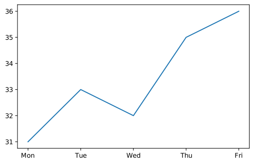
            Joins points with lines to show a trend over an ordered sequence, usually time. plt.plot(x, y): x and y must have the same length, or you get a ValueError. With only one list, plt.plot(y), the x values are 0, 1, 2 …

            Python
            import matplotlib.pyplot as plt
            days = ['Mon', 'Tue', 'Wed', 'Thu', 'Fri']
            temp = [31, 33, 32, 35, 36]
            plt.plot(days, temp)
            plt.show()
            Figure 1
            A line plot of temperature rising from 31 on Monday to 36 on Friday, with a dip on Wednesday.

            Several lines, colours, markers and a legend are in VIS.04 Customizing Plots.

            Bar graph: plt.bar() and plt.barh() #bar-graph

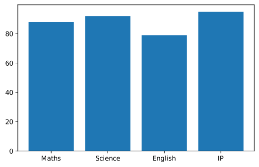
            Rectangles whose lengths compare separate categories, such as subjects, houses or cities. plt.bar(x, height) draws vertical bars: the first list gives the categories, the second gives the bar heights.

            Python
            import matplotlib.pyplot as plt
            subjects = ['Maths', 'Science', 'English', 'IP']
            marks = [88, 92, 79, 95]
            plt.bar(subjects, marks)
            plt.show()
            Figure 1
            A bar graph of marks in the default blue: Maths 88, Science 92, English 79, IP 95.

            Width, colours and edges

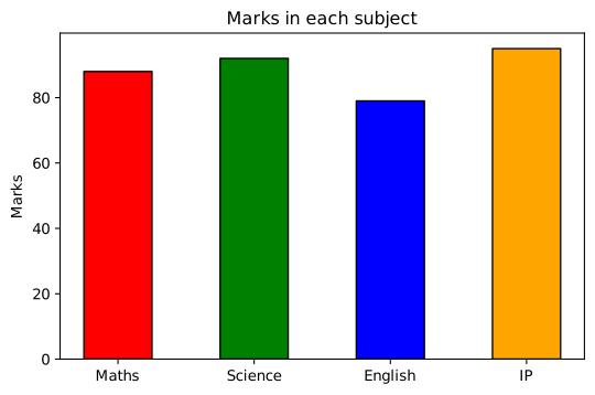
            width sets how wide each bar is (default 0.8; 1 makes bars touch). color can be one colour for all bars or a list with one colour per bar. edgecolor draws an outline.

            Python
            import matplotlib.pyplot as plt
            subjects = ['Maths', 'Science', 'English', 'IP']
            marks = [88, 92, 79, 95]
            plt.bar(subjects, marks, width=0.5,
                    color=['red', 'green', 'blue', 'orange'],
                    edgecolor='black')
            plt.ylabel('Marks')
            plt.title('Marks in each subject')
            plt.show()
            Figure 1
            Narrower bars, each a different colour (red, green, blue, orange) with black outlines, with a title and y-axis label.

            Horizontal bars: plt.barh()

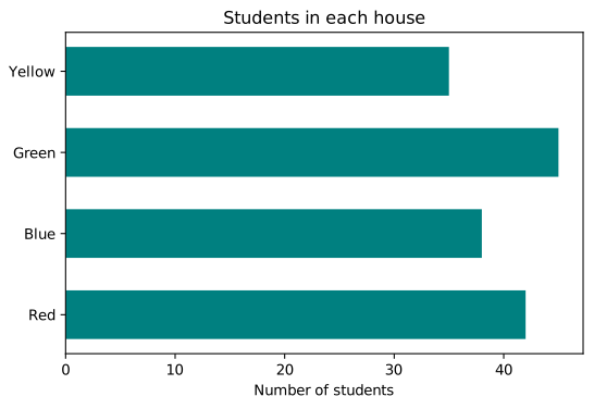
            plt.barh(y, width) draws the bars sideways. Categories go on the y-axis and lengths along the x-axis, so the axis labels swap: here the numbers need xlabel. Use it when category names are long or there are many of them.

            Python
            import matplotlib.pyplot as plt
            houses = ['Red', 'Blue', 'Green', 'Yellow']
            students = [42, 38, 45, 35]
            plt.barh(houses, students, height=0.6,
                     color='teal')
            plt.xlabel('Number of students')
            plt.title('Students in each house')
            plt.show()
            Figure 1
            Horizontal teal bars for the four houses: Red 42, Blue 38, Green 45, Yellow 35 students.
            Common mistake

            In barh() the words swap meaning: the second argument is the bar's length (its parameter is called width), and height= is the bar's thickness (default 0.8). In bar(), width= is the thickness.

            Two sets of bars side by side

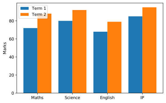
            To compare two terms for each subject, draw two bar() calls at slightly shifted positions. np.arange() gives the positions 0, 1, 2, 3; each set is moved 0.2 left or right and made 0.4 wide, so the pairs sit together. plt.xticks() then puts the subject names back under each pair.

            Python
            import matplotlib.pyplot as plt
            import numpy as np
            subjects = ['Maths', 'Science', 'English', 'IP']
            term1 = [72, 80, 68, 85]
            term2 = [88, 92, 79, 95]
            x = np.arange(len(subjects))      # 0, 1, 2, 3
            plt.bar(x - 0.2, term1, width=0.4, label='Term 1')
            plt.bar(x + 0.2, term2, width=0.4, label='Term 2')
            plt.xticks(x, subjects)
            plt.ylabel('Marks')
            plt.legend()
            plt.show()
            Figure 1
            Pairs of bars for each subject, Term 1 (blue) and Term 2 (orange), with subject names below and a legend.
            ParameterIn plt.bar(x, height, …)In plt.barh(y, width, …)
            First argumentCategories along the x-axisCategories along the y-axis
            Second argumentBar heightsBar lengths
            Bar thicknesswidth= (default 0.8)height= (default 0.8)
            colorOne colour, or a list of one colour per bar
            edgecolor, linewidthOutline colour and thickness
            labelName for the legend

            Histogram: plt.hist() #histogram

            Shows the distribution of numeric data. It splits the range into intervals called bins, counts how many values fall in each, and draws one bar per bin. The bars touch, because the bins are continuous. You give it the raw values, and it does the counting.

            bins as a number

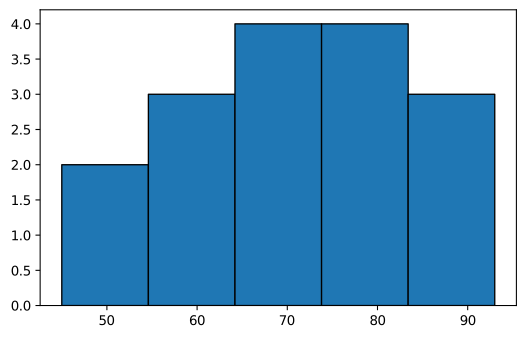
            bins=5 cuts the range from the smallest to the largest value into 5 equal bins. Here 45 to 93 gives bins 9.6 wide, holding 2, 3, 4, 4 and 3 scores. The default is 10 bins.

            Python
            import matplotlib.pyplot as plt
            scores = [45, 52, 58, 61, 63, 67, 68, 70,
                      72, 74, 75, 78, 81, 84, 88, 93]
            plt.hist(scores, bins=5, edgecolor='black')
            plt.show()
            Figure 1
            A histogram of 16 scores in 5 equal bins from 45 to 93, with counts 2, 3, 4, 4 and 3.

            bins as a list of edges

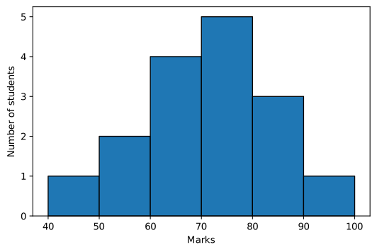
            A list gives the edges of the bins yourself, so they are round numbers like 40–50, 50–60 …. Each bin includes its left edge but not its right, except the last, which includes both. So 50 counts in 50–60, and 100 counts in 90–100. The counts here are 1, 2, 4, 5, 3 and 1.

            Python
            import matplotlib.pyplot as plt
            scores = [45, 52, 58, 61, 63, 67, 68, 70,
                      72, 74, 75, 78, 81, 84, 88, 93]
            edges = [40, 50, 60, 70, 80, 90, 100]
            plt.hist(scores, bins=edges, edgecolor='black')
            plt.xticks(edges)
            plt.xlabel('Marks')
            plt.ylabel('Number of students')
            plt.show()
            Figure 1
            A histogram with bins 40 to 100 in steps of 10, counts 1, 2, 4, 5, 3, 1, with the bin edges marked on the x-axis.

            weights: when the data is already counted

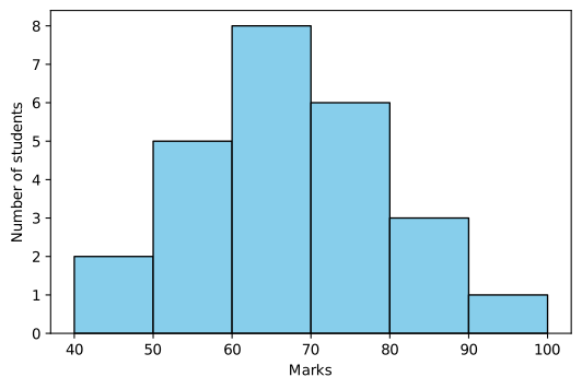
            Often you get a frequency table instead of raw marks: "2 students scored 40–50, 5 scored 50–60 …". Give one value from inside each range (here its middle) and pass the counts as weights. Each value is then counted as many times as its weight instead of once, so the bar heights are exactly the counts.

            Marks40–5050–6060–7070–8080–9090–100
            Students258631
            Python
            import matplotlib.pyplot as plt
            marks = [45, 55, 65, 75, 85, 95]    # middle of each range
            students = [2, 5, 8, 6, 3, 1]       # how many in each
            plt.hist(marks, bins=[40, 50, 60, 70, 80, 90, 100],
                     weights=students, edgecolor='black',
                     color='skyblue')
            plt.xlabel('Marks')
            plt.ylabel('Number of students')
            plt.show()
            Figure 1
            A histogram drawn from a frequency table with weights: bars of height 2, 5, 8, 6, 3 and 1 for the six mark ranges.

            Without weights, each of the six marks would be counted once, giving six bars of height 1. weights must be the same length as the data.

            Outline and running-total histograms

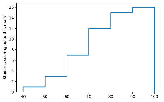
            histtype='step' draws only the outline. cumulative=True makes each bar include all the bins before it, so the last bar equals the total number of values: here 1, 3, 7, 12, 15, 16.

            Python
            import matplotlib.pyplot as plt
            scores = [45, 52, 58, 61, 63, 67, 68, 70,
                      72, 74, 75, 78, 81, 84, 88, 93]
            plt.hist(scores, bins=[40, 50, 60, 70, 80, 90, 100],
                     histtype='step', cumulative=True,
                     linewidth=2)
            plt.ylabel('Students scoring up to this mark')
            plt.show()
            Figure 1
            A cumulative step histogram rising 1, 3, 7, 12, 15, 16 across bins from 40 to 100.
            Parameter of plt.hist()MeaningExample
            x (first argument)The values to countscores
            binsA number of equal bins, or a list of edgesbins=5, bins=[0, 25, 50, 75, 100]
            weightsHow many times to count each valueweights=[2, 5, 8]
            rangeLowest and highest value to includerange=(40, 100)
            histtype'bar' (default), 'step' (outline), 'stepfilled'histtype='step'
            orientation'vertical' (default) or 'horizontal'orientation='horizontal'
            cumulativeEach bar adds all earlier binscumulative=True
            color, edgecolorFill and outline colouredgecolor='black'
            Line plotBar graphHorizontal barHistogram
            ShowsTrend over timeComparison of categoriesComparison, long namesDistribution of values
            You give itx and y valuesCategories and heightsCategories and lengthsRaw values (and bins)
            Functionplt.plot()plt.bar()plt.barh()plt.hist()
            Common mistake

            A bar graph and a histogram look alike, but a bar graph compares categories you name (gaps between bars, you give the heights), while a histogram counts how many values fall in each range (bars touch, it works out the heights).

            VIS.03 · Data Visualization

            Saving Plots

            12-IP

            plt.savefig('filename') saves the chart as an image file. The extension chooses the format: .png, .jpg, .pdf or .svg.

            Python
            import matplotlib.pyplot as plt
            days = ['Mon', 'Tue', 'Wed', 'Thu', 'Fri']
            temp = [31, 33, 32, 35, 36]
            plt.plot(days, temp)
            plt.savefig('temperature.png')    # save first
            plt.show()                        # then show
            Order matters

            Call savefig() before show(). Closing the chart window clears the figure, so saving afterwards gives a blank image.

            VIS.04 · Data Visualization

            Customizing Plots

            12-IP

            A chart should say what it shows. Add these after plotting and before show().

            Python
            import matplotlib.pyplot as plt
            days = ['Mon', 'Tue', 'Wed', 'Thu', 'Fri']
            delhi = [31, 33, 32, 35, 36]
            shimla = [22, 24, 23, 25, 27]
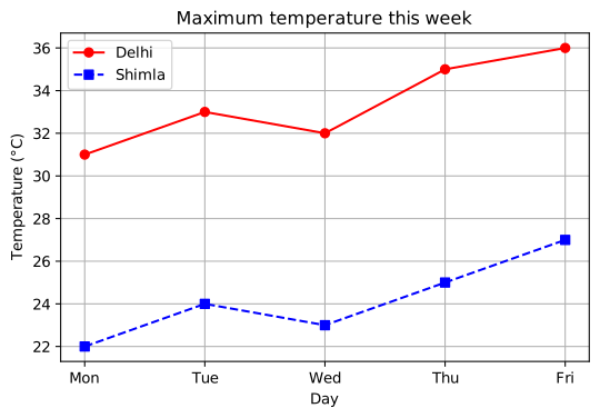
            plt.plot(days, delhi, label='Delhi',
                     color='red', marker='o')
            plt.plot(days, shimla, label='Shimla',
                     color='blue', linestyle='--', marker='s')
            plt.title('Maximum temperature this week')
            plt.xlabel('Day')
            plt.ylabel('Temperature (°C)')
            plt.legend()
            plt.grid(True)
            plt.show()
            Figure 1
            Two lines for Delhi (red, solid, circles) and Shimla (blue, dashed, squares) with a title, axis labels, legend and grid.

            Labels #label

            plt.xlabel('…') and plt.ylabel('…') name the axes. The label='…' argument inside plot() names a line for the legend.

            Title #title

            plt.title('…') puts a heading above the chart.

            Legend #legend

            plt.legend() shows a key matching each line to its label. Without labels, the legend is empty.

            Ticks: xticks() and yticks()

            Ticks are the small marks along an axis and the numbers or names written at them. Matplotlib chooses them for you. plt.xticks() and plt.yticks() let you choose where they go and what they say.

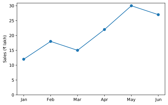
            plt.xticks(positions, labels) puts each label at a position. This plots months as 1 to 6, then shows month names there, and makes the y-axis go up in fives with range():

            Python
            import matplotlib.pyplot as plt
            sales = [12, 18, 15, 22, 30, 27]
            plt.plot([1, 2, 3, 4, 5, 6], sales, marker='o')
            plt.xticks([1, 2, 3, 4, 5, 6],
                       ['Jan', 'Feb', 'Mar', 'Apr', 'May', 'Jun'])
            plt.yticks(range(0, 35, 5))
            plt.ylabel('Sales (₹ lakh)')
            plt.show()
            Figure 1
            A line plot of monthly sales with Jan to Jun on the x-axis and y-axis ticks every 5 from 0 to 30.

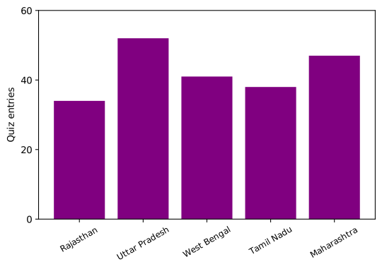
            Long category names overlap. rotation tilts the labels and fontsize makes them smaller. Giving only positions, like yticks([0, 20, 40, 60]), keeps the numbers as labels.

            Python
            import matplotlib.pyplot as plt
            teams = ['Rajasthan', 'Uttar Pradesh', 'West Bengal',
                     'Tamil Nadu', 'Maharashtra']
            entries = [34, 52, 41, 38, 47]
            plt.bar(teams, entries, color='purple')
            plt.xticks(rotation=30, fontsize=9)
            plt.yticks([0, 20, 40, 60])
            plt.ylabel('Quiz entries')
            plt.show()
            Figure 1
            A bar graph of quiz entries for five states with the state names tilted at 30 degrees and y-axis ticks at 0, 20, 40 and 60.
            You writeEffect
            plt.xticks([1, 2, 3])Ticks only at 1, 2, 3, labelled with those numbers
            plt.xticks([1, 2, 3], ['A', 'B', 'C'])Ticks at 1, 2, 3, labelled A, B, C. The two lists must be the same length
            plt.yticks(range(0, 101, 10))y ticks every 10 from 0 to 100
            plt.xticks(rotation=45)Keep the ticks, tilt the labels 45°
            plt.xticks(fontsize=8)Smaller tick labels
            plt.xticks([])Hide the x ticks altogether
            plt.xlim(0, 10) / plt.ylim(0, 100)Related: set where the axis starts and ends
            Exam tip

            xticks() changes the marks and labels along the axis; xlabel() is the one name of the whole axis. A question asking to "display month names on the x-axis" wants xticks().

            ArgumentChangesExample values
            colorLine or bar colour'red', 'g', 'blue', 'orange'
            linestyleLine pattern'-' solid, '--' dashed, ':' dotted, '-.' dash-dot
            linewidthLine thickness1, 2.5, 4
            markerSymbol at each point'o' circle, 's' square, '^' triangle, '*' star
            width / height (bars)Bar thickness in bar() / barh()0.4, 0.8
            edgecolorOutline of bars'black'
            bins, weights (hist)Intervals; how often each value counts5 or [0, 50, 100]; [2, 5, 8]
            Chapter practice · VIS

            Check your understanding

            Which plot?

            Show how a shop's sales changed month by month over a year.

            Compare the number of students in each house: Red, Blue, Green, Yellow.

            Show how many students scored 0–20, 21–40, 41–60 and so on in an exam.

            Compare the number of entries from 12 states with long names such as "Arunachal Pradesh".

            You are given only a table: "40–50: 2 students, 50–60: 5 students …" and must draw its histogram.

            Compare the daily temperatures of two cities on one chart.

            Self-check quiz

            Which function sets the title of a graph?
            Which line style value draws a dashed line?
            Each line has a label= but no legend appears. What is missing?
            In plt.barh(names, values, height=0.5), height=0.5 sets:
            Which shows the names Q1–Q4 at x positions 1–4?
            plt.hist([10, 30], bins=[0, 20, 40], weights=[4, 6]) draws bars of height:
            With bins=[0, 10, 20, 30], the value 20 falls in:
            The x-axis names overlap. Which tilts them?
            In plt.hist(data, bins=10), bins=10 means:
            Your score
            – / 9
            Answer every question to see your score.

            One-page revision

            plt.plot(x, y)line: trend
            plt.bar(x, h)bars: compare categories
            plt.barh(y, length)sideways bars; height= is thickness
            width=0.8default bar thickness in bar()
            color=[…]one colour per bar
            x ± 0.2, width=0.4two sets of bars side by side
            plt.hist(data, bins=n)distribution; n equal bins
            bins=[40, 50, …]your own edges; left edge included
            weights=[…]count each value that many times
            histtype='step' · cumulativeoutline · running total
            plt.xticks(pos, labels)choose tick positions and names
            xticks(rotation=45)tilt long labels
            xlabel · ylabel · titlename the axes and chart
            label= + legend()key for several lines
            color · linestyle · marker'r' · '--' · 'o'
            plt.savefig('a.png')save, before show()
            plt.show()display, last